When Will Evolution Outperform Local Search?

January 31, 2016January 10, 2019 Keki2 Comments

Recombinative evolution will outperform local search on fitness functions that have a property called deep contingency. In this blog post I will:

Present a fitness function possessing the property in question and empirically show that a genetic algorithm handily outperforms simulated annealing.
Argue that the presented problem is a difficult one, and the non-trivial computation performed by the genetic algorithm is just what’s needed.
Explain why simulated annealing, and indeed, local search of any kind, is the wrong way to approach the problem presented.

This is going to be a lengthy post, and you are welcome to jump to the punch. First, I want to explain why it has taken till now to procure a whitebox optimization problem on which a genetic algorithm outperforms simulated annealing. The short story is that we did not, till recently, have good theories about the computational power of recombinative evolution.

Here’s the long story:

Logical Positivism vs the Scientific Method in Genetic Algorithmics

The genetic algorithm owes its form to biomimicry, not derivation from first principles. So, unlike the workings of conventional optimization algorithms, which are typically apparent from the underlying mathematical derivations, the workings of the genetic algorithm require elucidation. Attempts to explain how genetic algorithms work can be divided in two: those based to a lesser or greater extent on the scientific method, and those that reject the scientific method in favor of logical positivism. Continue reading “When Will Evolution Outperform Local Search?” →

Evolutionary Optimization of Independent Deeply Contingent Components Happens in Parallel

February 10, 2016March 27, 2017 KekiLeave a comment

In my last post, I introduced the notion of deep contingency and contrasted it with deep hierarchy—the hypothesized property of fitness functions that genetic algorithms purportedly exploit. Here I provide evidence that recombinative evolution can optimize multiple deeply contingent components in parallel. Specifically, I generalize the contingent parities function presented in the previous post (which you should read first) and examine the performance of a simple genetic algorithm on an instance of the generalized problem. For the sake of comparison, the behavior of simulated annealing is also presented.

The pseudocode for a Contingent Parities Function with multiple components is given below:

mcpf-algo

The following figure shows the missteps of component 1 (in blue) and component 2 (in green) of a chromosome with maximal fitness in each generation when a simple genetic algorithm was applied to an contingent parities function with two components of order 2 and height 100. The y-coordinate of the green dots (representing the missteps of component 2) were dodged by +0.5 to reduce overlap. The maximal fitness in each generation is shown in red.

mcpf-ga

To regenerate this figure, clone the $\texttt{multicomponent-cpf}$ branch of this repository as follows:

git clone -b multicomponent-cpf https://github.com/burjorjee/royal-roads.git

Then execute the following python code:

import royalroads as rr
cpf = rr.ContingentParitiesFunction(order=2, height=100, numComponents=2)
rr.evolve(fitnessFunction=cpf,
          popSize=500,
          maxGens=1000,
          probMutation=0.004,
          sigmaScaling=True,
          sigmaScalingCoeff=0.5,
          useClamping=True,
          rngSeed=1,
          visualize=True)

The figure shows that the simple genetic algorithm optimizes both components of the contingent parities function concurrently. The maximal fitness achieved was 199.

A plot showing the behavior of simulated annealing on the same function follows below:

mcpf-sa

To regenerate this figure execute the following python code:

import royalroads as rr
cpf = rr.ContingentParitiesFunction(order=2, height=100, numComponents=2)
rr.anneal(fitnessFunction=cpf,
          epochsPerPeriod=500,
          numPeriods=1000,
          initFitnessDropOfOneAcceptanceProb=0.6,
          finalFitnessDropOfOneAcceptanceProb=0.01)

The maximal fitness achieved was 168.

Hypomixability Theory

July 12, 2015July 21, 2016 KekiLeave a comment

TL;DR: Computer scientists can say why the fast fourier transform is fast and why quicksort is quick. Yet when it comes to explaining what’s efficient about the computation that yielded ourselves, we currently draw a blank. Hypomixability theory provides the basis for an answer.

Run a population based recombinative evolutionary algorithm on a real world fitness function; until adaptation tapers off, you will find that the fitness of an offspring is, on average, lower than the mean fitness of its parents. You will find, in other words, that the average fitness of the population goes down after mixing (recombination) and up after selection. Selection, of course, makes sense—it increases average fitness. But why mixing? What sense does it make to recombine the genes of individuals with above average fitness, especially on epistatic landscapes where recombination is virtually guaranteed to lower average fitness? What computational purpose does mixing serve?

Hypomixability Theory explains why mixing makes computational sense and illuminates how mixing induced reductions in average fitness (the hypo in hypomixability) between parent and offspring populations can be indicative of room for adaptation. The theory is very parsimonious in its assumptions. It does not, for example, assume the presence of building blocks in the fitness landscape. Hypomixability Theory also comes with a prediction and proof of efficient computational learning in a recombinative evolutionary algorithm, making it the first, and currently only, computationally credible explanation for the “endless forms most beautiful and wonderful” that comprise the the sexually reproducing part of the biosphere. Our remarkable species included.

Paper: Efficient Hypomixability Elimination in Recombinative Evolutionary Systems

Explaining Sex, Adaptation, Speciation, and the Emergence of Genetic Modularity

March 2, 2015November 1, 2017 Kekiadaptation, emergence of modularity, foga 2015, learning juntas, learning parities, mixability, optimal bounds, PAC-Learning, parsimony, sex, speciation, unificationLeave a comment

To appear in the proceedings of the Foundations of Genetic Algorithms Conference, 2015

Hypomixability Elimination in Evolutionary Systems

Abstract: Hypomixability Elimination is an intriguing form of computation thought to underlie general-purpose, non-local, noise-tolerant adaptation in recombinative evolutionary systems. We demonstrate that hypomixability elimination in recombinative evolutionary systems can be efficient by using it to obtain optimal bounds on the time and queries required to solve a subclass $(k=7, \eta=1/5)$ of a familiar computational learning problem: PAC-learning parities with noisy membership queries; where $k$ is the number of relevant attributes and $\eta$ is the oracle’s noise rate. Specifically, we show that a simple genetic algorithm with uniform crossover (free recombination) that treats the noisy membership query oracle as a fitness function can be rigged to PAC-learn the relevant variables in $O(\log (n/\delta))$ queries and $O(n \log (n/\delta))$ time, where $n$ is the total number of attributes and $\delta$ is the probability of error. To the best of our knowledge, this is the first time optimally efficient computation has been shown to occur in an evolutionary algorithm on a non-trivial problem.

The optimality result and indeed the implicit implementation of hypomixability elimination by a simple genetic algorithm depends crucially on recombination. This dependence yields a fresh, unified explanation for sex, adaptation, speciation, and the emergence of modularity in evolutionary systems. Compared to other explanations, Hypomixability Theory is exceedingly parsimonious. For example, it does not assume deleterious mutation, a changing fitness landscape, or the existence of building blocks.

Efficiently Evo-learning Juntas With Membership Queries

September 3, 2013January 23, 2015 KekiComputational learning theory, evolutionary computation, genetic algorithm, implicit concurrency, learning juntasLeave a comment

Recently, I showed that a simple genetic algorithm with uniform crossover can solve a noisy learning 7-parity problem efficiently—in $O(n \textrm{ polylog}(n, \frac{1}{\epsilon}))$ time and $O(\textrm{polylog}(n, \frac{1}{\epsilon}))$ membership queries. Learning parities is a subclass of a more general problem—learning juntas—that is of considerable interest to computational learning theorists because it neatly abstracts the general problem of learning in the presence of large amounts of irrelevant information. This is a very common problem in practice. A good example comes, coincidentally, from the field of genetic epidemiology—learning the genetic loci participating in the penetrance of a particular disease. (More about this “coincidence” in a bit)

The implicit concurrency hypothesis posits that the efficient learning of relevant variables in the presence of large numbers of irrelevant variables is precisely what gives evolution its power; so, understandably, when I read about the learning juntas problem a few weeks ago (on this blog), I sensed the possibility of a connection. Formally, a $k$ -junta is a function $f$ over $n$ boolean variables, only $j\,\,(\leq k\leq n)$ of which matter (i.e. are relevant) in the determination of the output of $f$ . The $j$ relevant variables are said to be the juntas of $f$ , and the function $f$ is completely characterized by its juntas and by a hidden boolean function $h$ over $j$ inputs. The output of $f$ is just the output of $h$ on the values of the $j$ relevant variables of $f$ (the values of the irrelevant variables are simply ignored). The problem of identifying the relevant variables is called the learning juntas problem.

Observe how this problem abstracts the genetic epidemiology problem mentioned above. The junta are the genetic loci participating in the presence/absence of the disease. The hidden function specifies which configurations of alleles at these loci cause the disease, and which ones do not. The problem of learning the relevant loci is the problem of learning juntas. Also note that the learning juntas problem generalizes the learning parities problem straightforwardly. Whereas the hidden function in the case of learning parities must be the parity function, the hidden function in the case of learning juntas can be any boolean function over the juntas.

Here is an evolution based algorithm, written in Python, that learns juntas given a membership query oracle. And here is a tutorial on its usage. For any value of $k$ , the theory of implicit concurrency suggests that the $k$ -junta for which it is hardest for a genetic algorithm to learn one or more relevant attributes (Mossel et al observed in Learning Juntas that to crack the problem, asymptotically speaking, one only needs to find a single relevant attribute) is the $k$ -junta with a hidden parity function over $k$ variables. This insight and my previous work on learning parities suggests that the evolutionary algorithm presented can learn the relevant attributes of $k$ -juntas with small $k$ in $O(n\textrm{ polylog}(n, \frac{1}{\epsilon}))$ time and $O(\textrm{polylog}(n, \frac{1}{\epsilon}))$ queries.

Implications for the Neo-Darwinian Synthesis

It seems like more than a coincidence that

The Learning Juntas problem abstracts the genetic epidemiology problem mentioned earlier
Evolutionary computation can efficiently solve the Learning Juntas problem for small numbers of juntas.

One is hard pressed not to hypothesize that evolution takes the form it takes precisely because this form allows it to solve a problem that is similar to the genetic epidemiology problem in all significant ways, save two :

The problem is to learn the genetic loci participating in fitness/hotness not disease penetrance (often the same loci, but by no means always)
Unlike computational geneticists, evolution has access to an active oracle.

Given the straightforwardness of this idea it may seem odd that it has not been forthcoming from Evolutionary Biology itself; that is until one realizes that a deep-rooted practice in Population Genetics actively steers theorists away. A vestige from the days before computers, when pen, paper, and mathematics was all one had, the conflation of the unit of inheritance with the unit of selection casts a long shadow. More about this in Sections 2.4.1 and 5.1 of my dissertation.

What now?

Despite the routine use of evolutionary algorithms in science and engineering, computer scientists have been unable to give a straight answer to a simple question: “Is there anything computationally efficient about evolution?” This question can now be answered in the affirmative. Recombinative evolutionary algorithms are capable of efficiently solving a broad, non-trivial problem: Learning $k$ -Juntas with membership queries when $k$ is small.

While fascinating from a biological perspective, this answer is not entirely satisfying to the engineer in me because there are conventional algorithms that solve the problem under consideration as efficiently; for example, the binary search algorithm due to Blum and Langley described in Section 5 of the paper by Mossel et al. A more involved algorithm due to Feldman solves the problem almost as efficiently, and does so non-adaptively and in the presence of random persistent classification error.

Have modern ML techniques eclipsed evolution at the very thing it is good at?

I have a hunch that the answer is “no”. It would be fantastic to find generalizations of the learning juntas with membership queries problem that are more difficult for conventional algorithms, but remain efficiently solvable by evolution.

Relevant Computational Learning Theory papers
R.J. Lipton
[web] The Learning Juntas Problem
(An excellent introduction to the Learning Juntas problem)

E. Mossel, R. O’donnell, and R. Servedio
[pdf] Learning Juntas,
(Section 3.1 is especially relevant if you want to reverse engineering the posted Python algorithm)

A. Blum, L. Hellerstein, and N. Littlestone
[pdf] Learning in the Presence of Finitely or Infitely Many Irrelevant Attributes

V. Feldman
[pdf] Attribute-Efﬁcient and Non-adaptive Learning of Parities and DNF Expressions

Relevant papers on Implicit Concurrency
K.M. Burjorjee
[pdf] The Fundamental Learning Problem that Genetic Algorithms with Uniform Crossover Solve Efficiently and Repeatedly as Evolution Proceeds

K.M. Burjorjee
[pdf] Explaining Optimization in Genetic Algorithms with Uniform Crossover

Relevant papers on genetic epidemiology
J.H. Moore, L.W. Hahn, M.D. Ritchie, T.A. Thornton, and B.C. White
[web] Routine Discovery of Complex Genetic Models using Genetic Algorithms

J.H. Moore
[web] The ubiquitous nature of epistasis in determining susceptibility to common human diseases

Last Updated: September 18, 2013

Theoretical Bonafides For Implicit Concurrency

July 21, 2013August 10, 2015 Kekibuilding block hypothesis, decimation, genetic algorithms, implicit concurrency, learning parities, survey propagation, what are GAs good for?Leave a comment

A commonly asked question since the early days of evolutionary computation is “What are Genetic Algorithms good for?” What, in other words, is the thing that genetic algorithms (GAs) do well? The prevailing answer for almost two decades was “Hierarchical Building Block Assembly”. This answer, which goes by the name of the building block hypothesis, generated tremendous excitement in its day and helped jumpstart the field of genetic algorithmics. However it fell into disrepute during the ’90s because of a lack of theoretical support and (more damningly) anomalies in the empirical record.

Since then, The Question (“What are GAs good for?”) has gone unanswered—or, to be precise, remains poorly answered—The Building Block Hypothesis continues on as a placeholder in textbooks. More recently, The Question is increasingly going unasked by evolutionary computation theorists, in large part because EC theorists are now wary of entertaining claims about genetic algorithms that cannot be formally deduced, and because Genetic algorithms used in practice (ones with finite but non-unitary recombinative populations) have proven frustratingly resistant to conventional analytic approaches.

The following paper squares off with Das Question, and for genetic algorithms with uniform crossover (UGAs), ventures an answer: Implicit Concurrent Multivariate Effect Evaluation—implicit concurrency for short—is what UGAs are good for. Implicit concurrency is compared with implicit parallelism (the “engine of optimization” according to the building block hypothesis), and the former is revealed to be more powerful.

Empirical evidence for implicit concurrency can be found here and here. And additional empirical evidence is easily obtained for one-off problem instances—just run a genetic algorithm on the appropriately chosen instance. The paper below takes a different tack. It establishes theoretical support (across an infinite set of problem instances) for the claim that implicit concurrency is a form of efficient computational learning. It achieves this end by demonstrating that implicit concurrency can be used to obtain low bounds on the time and query complexity of a UGA based algorithm that solves a constrained version of a well recognized problem from the computational learning literature: Learning parities with a noisy membership query oracle.

The difficulty of formally analyzing genetic algorithms is circumvented with an empirico-symmetry-analytic proof comprised of

A formal part (no knowledge of genetic algorithms required)
An accessible symmetry argument
A simple statistical hypothesis testing based rejection of a null hypothesis with very high significance $p<10^{-100}$

The paper is here:
The Fundamental Learning Problem that GAs with UX Solve Efficiently and Repeatedly as Evolution Proceeds

The code used to conduct the experiment is here:
https://github.com/kburjorj/speedyGApy/blob/master/soda14.py

Parallel Effect Search in Genetic Algorithms

March 24, 2013August 24, 2016 Kekigenetic algorithms, global optimization, implicit concurrency, machine learningLeave a comment

The thing genetic algorithms do efficiently—Parallel Effect Search —is not difficult to describe or demonstrate. It’s been under our noses since schemata and schema partitions were defined as concepts, but for various reasons, which I won’t get into here, it’s not widely appreciated. This blog post provides a quick introduction. For a more in depth treatment check out my FOGA 2013 paper Explaining Optimization in Genetic Algorithms with Uniform Crossover (slides here).

Schema Partitions and Effects

Let’s begin with a quick primer on schemata and schema partitions. Let $S=\{0,1\}^\ell$ be a search space consisting of binary strings of length $\ell$ . Let $\mathcal I$ be some set of indices between $1$ and $\ell$ , i.e. $\mathcal I\subseteq\{1,\ldots,\ell\}$ . Then $\mathcal I$ represents a partition of $S$ into $2^{|\mathcal I|}$ subsets called schemata (singular schema) as in the following example: suppose $\ell=4$ , and $\mathcal I=\{1,3\}$ , then $\mathcal I$ partitions $S$ into four schemata:

$0*0* = \{0000, 0001, 0100, 0101\}$

$0*1* = \{0010, 0011, 0110, 0111\}$

$1*0* = \{1000, 1001, 1100, 1101\}$

$1*1* = \{1010, 1011, 1110, 1111\}$

where the symbol $*$ stands for ‘wildcard’. Partitions of this type are called schema partitions. As we’ve already seen, schemata can be expressed using templates, for example, $0*1*$ . The same goes for schema partitions. For example $\#*\#*$ denotes the schema partition represented by the index set $\mathcal I$ . Here the symbol $\#$ stands for ‘defined bit’. The order of a schema partition is simply the cardinality of the index set that defines the partition (in our running example, it is $|\mathcal I| = 2$ ). Clearly, schema partitions of lower order are coarser than schema partitions of higher order.

Let us define the effect of a schema partition to be the variance of the average fitness values of the constituent schemata under sampling from the uniform distribution over each schema. So for example, the effect of the schema partition $\#*\#*=\{0*0*\,,\, 0*1*\,,\, 1*0*\,,\, 1*1*\}$ is

$\frac{1}{4}\sum\limits_{i=0}^1\sum\limits_{j=0}^1(F(i*j*)-F(****))^2$

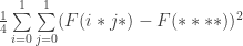
where the operator $F$ gives the average fitness of a schema under sampling from the uniform distribution.

You’re now well poised to understand Parallel Effect Search. Before we get to a description, a brief detour to provide some motivation: We’re going to do a thought experiment in which we examine how effects change with the coarseness of schema partitions. Let $[\mathcal I]$ denote the schema partition represented by some index set $\mathcal I$ . Consider a search space $S=\{0,1\}^\ell$ with $\ell=10^6$ , and let $\mathcal I =\{1,\ldots,10^6\}$ . Then $[\mathcal I]$ is the finest possible partition of $S$ ; one where each schema in the partition has just one point. Consider what happens to the effect of $[\mathcal I]$ as we start removing elements from $\mathcal I$ . It should be relatively easy to see that the effect of $[\mathcal I]$ decreases monotonically. Why? Because we’re averaging over points that used to be in separate partitions. Don’t proceed further until you convince yourself that coarsening a partition tends to decrease its effect.

Finally, observe that the number of schema partitions of order $o$ is ${\ell \choose o}$ . So for $\ell = 10^6$ , the number of schema partitions of order 2,3,4 and 5 are on the order of $10^{11}, 10^{17}, 10^{23}$ , and $10^{28}$ respectively. The take away from our thought experiment is this: while a search space may have vast numbers of coarse schema partitions, most of them will have negligible effects (due to averaging). In other words, while coarse schema partitions are numerous, ones with non-negligible effects are rare.

So what exactly does a genetic algorithm do efficiently? Using experiments and symmetry arguments I’ve demonstrated that a genetic algorithm with uniform crossover can sift through vast numbers of coarse schema partitions in parallel and identify partitions with non-negligible effects. In other words, a genetic algorithm with uniform crossover can implicitly perform multitudes of effect/no-effect multifactor analyses and can efficiently identify interacting loci with non-negligible effects.

Let’s Play a Game

It’s actually quite easy to visualize a genetic algorithm as it identifies such loci. Let’s play a game. Consider a stochastic function that takes bitstrings of length 200 as input and returns an output that depends on the values of the bits of at just four indices. These four indices are fixed; they can be any one of the ${\ell \choose 4}$ combinations of four indices between between 1 and 200. Given some bitstring, if the parity of the bits at these indices is 1 (i.e. if the sum of the four bits is odd) then the stochastic function returns a value drawn from the magenta distribution (see below). Otherwise, it returns a value drawn from the black distribution. The four indices are said to be pivotal. All other indices are said to be non-pivotal.

parityDistribs

As per the discussion in the first part of this post, the set of pivotal indices is the dual of a schema partition of order 4. Of all the schema partitions of order 4 or less, only this partition has a non-zero effect. All other schema partitions of order 4 or less have no effect. (Verify for yourself that this is true) In other words parity seems like a Needle in a Haystack (NIAH) problem—a problem, in other words, that requires brute force.

Now for the rules of the game: Say I give you query access to the stochastic function just described, but I do not tell you what four indices are pivotal. You are free to query the function with any bitstring 200 bits long as many times as you want. Your job is to recover the pivotal indices I picked, i.e. to identify the only schema partition of order 4 or less with a non-negligible effect.

Take a moment to think about how you would do it? What is the time and query complexity of your method?

What “Not Breaking a Sweat” Looks Like

The animation below shows what happens when a genetic algorithm with uniform crossover is applied to the stochastic function just described. Each dot displays the proportion of 1’s in the population at a locus. Note that it’s trivial to just “read off” the proportion of 0s at each locus. The four pivotal loci are marked by red dots. Of course, the genetic algorithm does not “know” that these loci are special. It only has query access to the stochastic function.

As the animation shows, after 500 generations you can simply “read off” the four loci I picked by examining the proportion of 1s to 0s in the population at each locus. You’ve just seen Parallel Effect Search in action. The chromosome size in this case is 200, so there are ${200 \choose 4}$ possible combinations of four loci. From all of these possibilities, the genetic algorithm managed to identify the correct one within five hundred generations.

Let’s put the genetic algorithm through it’s paces. I’m going to tack on an additional 800 non-pivotal loci while leaving the indices of the four pivotal loci unchanged. Check out what happens:

[Note: more dots in the animation below does not mean a bigger population or more queries. More dots just means more loci under consideration. The population size and total number of queries remain the same]

So despite a quintupling in the number of bits, entailing an increase in the number of coarse schema partitions of order 4 to ${1000 \choose 4}$ , the genetic algorithm solves the problem with no increase in the number of queries. Not bad. (Of course we’re talking about a single run of a stochastic process. And yes, it’s a representative run. See chapter 3 of my dissertation to get a sense for the shape of the underlying process)

Let’s take it up another notch, and increase the length of the bitstrings to 10,000. So now we’re looking at ${10000 \choose 4} \sim 10^{18}$ combinations of four loci. That’s on the order of a million trillion combinations. This time round, let’s also change the locations of the 4 pivotal loci. Will the genetic algorithm find them in 500 generations or less?

How’s that for not breaking a sweat? Don’t be deceived by the ease with which the genetic algorithm finds the answer. This is not an easy problem.

To run the experiments yourself download speedyGApy, and run it with

python speedyGA.py --fitnessFunction seap --bitstringLength <big number>

noting that the increase in “wall clock” time between generations as you increase bitstringLength is due to an increase in the running time of everything (including query evaluation). The number of queries (i.e. number of fitness evaluations), however, stays the same. To learn how a genetic algorithm parlays parallel effect search into a general-purpose global search heuristic called hyperclimbing, read my FOGA 2013 paper Explaining Optimization in Genetic Algorithms with Uniform Crossover (slides here).

FOGA 2013 Slides

January 20, 2013May 15, 2015 Kekifoga 2013, genetic algorithm, hyperclimbing, hyperscapes, implicit concurrency, maxsat, survey propagation, uniform crossover2 Comments

Optimization by Genetic Algorithms with uniform crossover is one of the deep mysteries of Evolutionary Computation. At first glance, the efficacy of uniform crossover, an extremely disruptive form of variation, makes no sense. Yet, genetic algorithms with uniform crossover often outperform genetic algorithms with variation operators that induce tight linkage between genetic loci.

At the Foundations of Genetic Algorithms Conference XII (January 16-20, Adelaide), I proposed an explanation for the efficacy of uniform crossover. The hypothesis presented posits that genetic algorithms with uniform crossover implement an intuitive, general purpose, global optimization heuristic called Hyperclimbing extraordinarily efficiently. The final version of the paper is available here. A generalization of the Hyperclimbing Hypothesis that explains optimization by genetic algorithms with less disruptive forms of crossover appears in my dissertation.

The presentation contains several animations, such as the one below, that serve as proof of concept for the Hyperclimbing Hypothesis. To view the animations, click on the “Watch On YouTube” links in the slides above or just download the presentation (93 Mb) and view it in Adobe Acrobat Reader. Note: the pdf reader in Chrome will not display the animations.

Download SpeedyGApy to run the experiments yourself (easy, and highly recommended).

SpeedyGA Ported to Python

January 20, 2013April 6, 2013 KekiLeave a comment

Today, I ported SpeedyGA from Matlab to Python. SpeedyGApy is a configurable, single-file, barebones, vectorized, numpy + matplotlib based genetic algorithm that rips.

SpeedyGApy Github Repo

The following video shows the kind of animation that gets displayed when speedyGA is run on a staircase function. Animations like this one serve as proof-of-concept for the Hyperclimbing Hypothesis, a new explanation for optimization in genetic algorithms with uniform crossover. Once you’ve downloaded speedyGApy, you can run this, and other experiments for yourself with the following command:

$ python speedyGA.py --fitnessFunction staircase

Generative Fixation

November 18, 2011February 13, 2016 KekiLeave a comment

One of the mainstays of human engineering is the idea of hierarchical assembly—the assembly of useful low level modules (a.k.a. building blocks) into useful modules at higher levels. Artifacts ranging from nuclear submarines to enterprise software are all constructed in this fashion. The building block hypothesis holds that genetic algorithms also construct solutions using hierarchical assembly, and that the basic building blocks used by these algorithms are short chromosomal snippets that confer above average fitness. Tantalizing as this hypothesis may be, it is based on strong assumptions about the distribution of fitness over a search space. I’ve criticized these assumptions in my dissertation and have proposed a different hypothesis based on weaker assumptions. This alternate hypothesis is grounded in a different metaphor—generative fixation.

Though not as ubiquitously recognizable as hierarchical assembly, generative fixation underlies progress in many areas. Like in the video industry for instance, which only really took off once the VHS/Betamax war had run its course. The “fixation” of VHS within this industry in essence generated new opportunities for advancement. For example, it permitted the development of the video rental business, which brought films from the back rooms of studio houses into living rooms everywhere. Had the tussle between VHS and Betamax continued, many of these opportunities might not have presented themselves. The economics of supporting two formats simultaneously would have been economically crippling for the fledgling industry.

VHS v. Betamax was a case where two contestants competed for dominance along a single dimension—the format accepted by video players. Consider a scenario consisting of multiple dimensions and multiple contestants in each dimension. Suppose, moreover, that no contestant in any dimension is outright superior. That is, the superioriority/non-superiority of the contestants in each dimension is dependent on the state of the contests in the other dimensions. This scenario describes the most commonly arising situation in natural evolution. Here, the “dimensions” are genetic loci, and the “contestants” are alleles. (Statistically, the scenario just described is more likely than one where one or more locus has an allele that is superior regardless of the frequencies of the alleles at other loci.)

The danger in such cases is that progress will stall because no contestant will come to dominate its dimension. The generative fixation hypothesis holds that in a system undergoing recombinative evolutionary dynamics, progress will continue. Although no locus has an allele that is outright superior, a small number of alleles belonging to different dimensions that play nice together (i.e. confer above average fitness as a group) will come to dominate their respective dimensions. In doing so, they will set the stage for the next multi-dimensional contest over the remaining dimensions. And so on.

I’ve demonstrated the genetic algorithm’s ability to scaleably identify and fix synergistic sets of unlinked non-competing alleles in a recent manuscript and in my dissertation.

evorithmics

Understanding and Harnessing the Computational Power of Evolution