In this blog entry I’d like to showcase just one of a number of remarkable findings that comprise the basis for the generative fixation hypothesis—a new explanation for the adaptive capacity of recombinative genetic algorithms.

Consider the following stochastic function which takes a bitstring of length as input and returns a real value as output.

fitness(bitstring)
  accum = 0
  for i = 1 to 4
     accum = accum + bitstring[pivotalLoci[i]]
  end
  if accum is odd
     return a random value from normal distribution N(+0.25,1)
  else
     return a random value from normal distribution N(-0.25,1)
  end

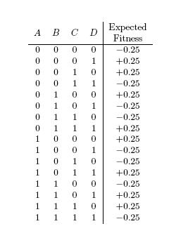
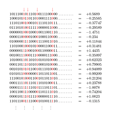
The variable pivotalLoci is an array of four distinct integers between 1and which specifies the location of  four loci—let’s call them A, B, C, D—of an input bitstring that matter in the determination the bitstring’s fitness. These four loci are said to be pivotal. The other bits of the input bitstring do not matter in the determination of the bitstring’s fitness, and are said to be non-pivotal. Given some input bitstring, if the parity of the bits at the pivotal loci is odd, then the fitness of the bitstring is drawn from a normal distribution with mean 0.25, and variance 1 (the magenta distribution; see below). Otherwise the fitness is drawn from a normal distribution with mean -0.25, and variance 1 (the black distribution).

The expected fitness of each of the 16  “genotypes” of ABCD is shown below.

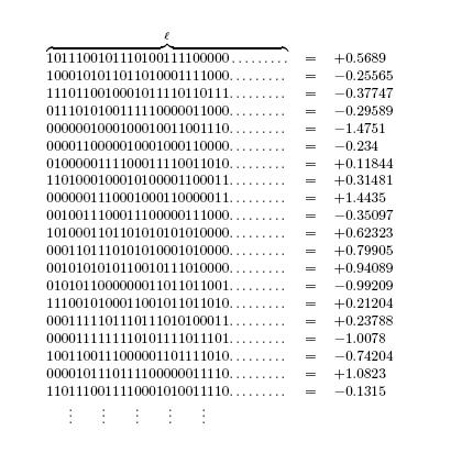
The following figure depicts the result of querying the fitness function with randomly generated bitstrings of length .

The next figure shows the locations of the pivotal loci A, B, C, D in this hypothetical scenario.

Consider the problem of classifying loci as pivotal or non-pivotal given only query access to the fitness function. This problem is closely related to the problem of finding the effective attributes of a parity function studied by Uehara et al.  [1,2]. One big difference is the presence of a stochastic element in the problem currently under consideration. Before reading further, I invite you to think of an algorithm that can solve this problem relatively robustly (with not more than, say, a 0.005 chance of misclassification per locus).

The naive approach would be to adopt a scanning strategy in which all combinations of four loci are visited. (Observe that visiting loci in combinations of three or less will not work). Suppose = 500,000; that’s approximately 6.25×10²² combinations. Even if it were possible to visit a million combinations per second, it would still take approximately two billion years to visit all such combinations.

It turns out that a genetic algorithm can be used to tackle this problem far more cheaply.

Suppose = 200 and pivotalLoci = [7 90 131 198]. The animation below shows the behavior of a simple genetic algorithm with uniform crossover (described in the materials and methods section of my dissertation) on the fitness function just described. Each frame in this animation shows the one-frequency of each locus (i.e. the frequency of the bit 1 at each locus) in a single generation. By extension, the frequency of the bit 0 at each locus is also on display. The red dots mark the positions of the pivotal loci. The blue dots mark the positions of non-pivotal loci.

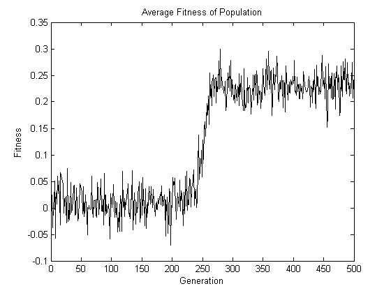
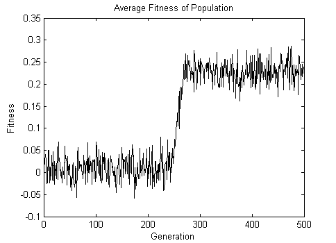
Observe that the red dots diverge to the top or bottom of the plot, whereas the blue dots remain in the middle. After 500 generations, the location of the pivotal loci A, B, C, and D can simply be “read off” by examining the one-frequency of each of the 200 loci in the final population. Note also that the genotype of ABCD that goes to fixation is 1011. This genotype has odd parity, which explains the increase in the average fitness of the population shown in the following figure.

Now for the two-part punchline. First, there is nothing special about the location of the four pivotal loci. In other words, the expected number of generations required for the four red dots to diverge to the top or bottom of the plot remains the same regardless of the location of these dots. Second, there is nothing special about = 200. In other words, the behavior of the red dots will be unaffected by the number of blue dots present, and each blue dot will have the same behavior regardless of the total number of blue dots. Both these conclusions can be arrived at by appreciating the symmetries present when is applied to the fitness function described above (or rather, to the class of fitness functions described). Readers looking for a more rigorous treatment are referred to chapter 3 of my dissertation.

The animation below shows the result of applying to the fitness function when = 1000. The array pivotalLoci remained unchanged at [7 90 131 198].

The average fitness of the population over 500 generations is shown below.

The final animation shows the result of applying to the fitness function when = 10000. In this case, the array pivotalLoci was set to [2000 2681 6892 9520].

The average fitness of the population over 500 generations is shown below.

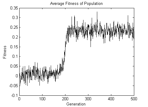
Note that in keeping with the assertions made above, the number of generations it takes for the red dots to diverge remains approximately the same despite an increase in by two orders of magnitude.

I hope the experience of watching evolutionary computation in action sparks your curiosity about the generative fixation hypothesis. Feel free to email me your questions and comments.

Click here to see the Matlab script used to generate the results presented above.

[1] Uehara, Tsuchida, and Wegener. Optimal attribute-efficient learning of disjunction, parity and threshold functions. In EUROCOLT: EUROCOLT, European Conference on Computational Learning Theory, EuroCOLT,. LNCS, 1997.

[2] Uehara, Tsuchida, and Wegener. Identication of partial disjunction, parity, and threshold functions. TCS: Theoretical Computer Science, 230, 2000.